Industrial process tomography
Industrial process tomography
In process tomography, industrial processes are monitored non-intrusively using boundary measurements. Typical applications of process tomography include imaging of mass transport, chemical reactions and mixing and separation processes. Tomographic images can be utilized in on-line monitoring, design and control of industrial processes.
The research in the Computational physics and inverse problems group covers both instrumentation issues and image reconstruction in process tomography. The main research topics include imaging of mixing and separation processes based on electrical resistance tomography (ERT), estimation of velocity fields based on electromagnetic flow tomography (EMFT), hardware design in EMFT and EIT and development of image reconstruction approaches for ERT, EMFT and electrical capacitance tomography (ECT).
Below there are some simulation results of EMFT reconstructions. A measurement system has also been built for collecting real data in laboratory environments.
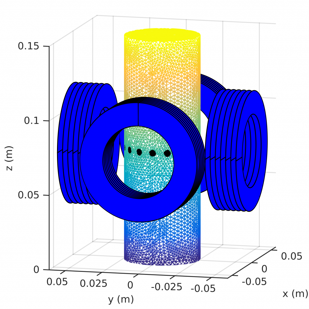
Figure: Simulation geometry of an EMFT system with four coils and 16 electrodes marked with black circular patches.
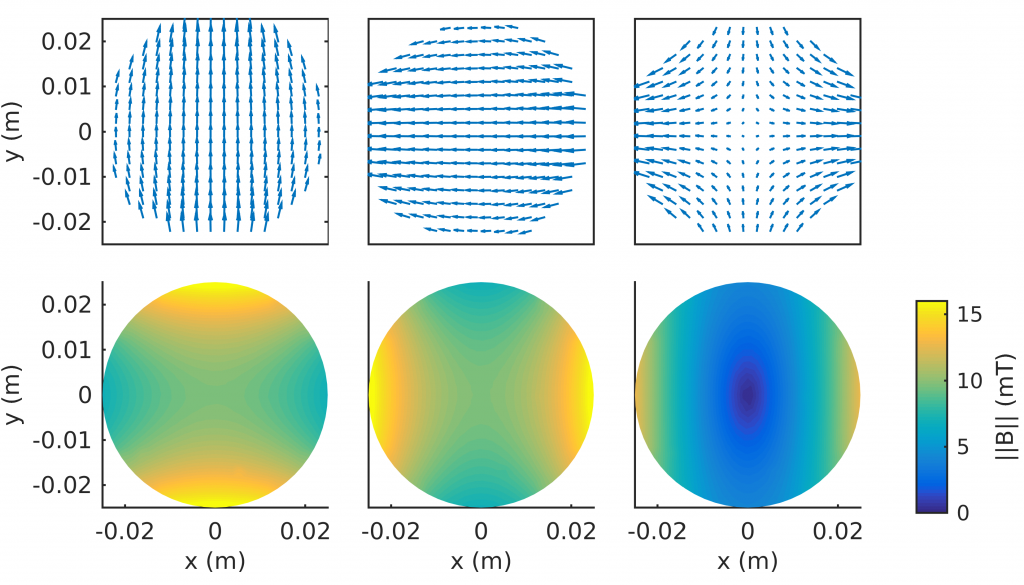
Figure: Vector plots (top row) and amplitudes (bottom row) of different magnetic field excitations at the 2D measurement plane. Excitations from left to right: nearly uniform excitation along y-axis (E1), nearly uniform excitation along x-axis (E2) and anti-Helmholtz excitation (E3).
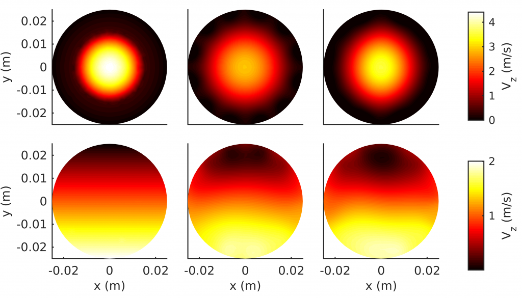
Figure: True z-components of the velocity fields (left column) used to simulate the voltage measurements and the estimated z-components of the velocities using two excitations E1 and E2 (middle column) and using E1 and E3 (right column). Top row is an annular and bottom row a stratified velocity field.
Contact
Past and present collaborators
- Professor, Daniel Sbarbaro, University of Concepcion, Chile
- Professor, Manuchehr Soleimani, University of Bath, UK
- Professor, Gary Lucas, University of Huddersfield, UK
- Professor, Uwe Hampel, HZDR, Germany
- Professor, Tuomas Koiranen, Lappeenranta University of Technology, Finland
Spin-offs
- A spin-off company Numcore Ltd was founded in 2007 by some researchers from the Computational physics and inverse problems group to commercialize research results related to EIT and process tomography. Numcore was sold to Outotec Oyj in 2012.
- A spin-off company Rocsole Ltd was founded in 2012 by some researchers from the Computational physics and inverse problems group to commercialize research results related to ECT and process tomography.